Tropical Variables
We use different variables to track and analyze equatorial wave activity.
Outgoing Longwave Radiation (OLR): OLR is the easiest way to track the convective components of convectively coupled equatorial waves (CCEWs). OLR is a measure of the outgoing longwave radiation at the top of the atmosphere (W/m^2) and can be used as a proxy for large areas of cloudiness/convection in the tropics. It should be interpreted in a large-scale sense. There is no guarantee that rain exists underneath areas where OLR values indicate convection. Negative (low) OLR anomalies/values are proxies for active convection and positive (high) OLR anomalies/values are proxies for suppressed convection because clouds reduce the amount of longwave radiation that escapes.
Zonal Wind: zonal wind is a good way to track the dynamic structures of CCEWs. Recall that many of the waves, such as the MJO and Kelvin waves, have strong easterly (ahead) and westerly (behind) phases.
Meridional Wind: meridional wind is especially good for tracking mid-latitude wave trains. Imagine a trough/ridge pattern. The meridional wind is southerly between trough/ridge combinations and northerly between ridge/trough combinations.
Velocity Potential velocity potential is a large scale field which is a broad measure of divergence. (The divergent [irrotational] wind is equal to the gradient of the velocity potential.) Since this is an integral of the divergent wind, it is a smoother field than the divergent wind, or simply divergence, itself. Areas of upper level divergence can be associated with the active convective areas of CCEWs and areas of upper level convergence can be associated with the suppresed convective parts of CCEWs. Note that velocity potential can make CCEWs appear to be more planetary scale in nature than they actually are – and this problem is worse for low wavenumber (longer) waves. People often consider a strong MJO as creating a planetary Wave-1 structure.
Real Time Diagnosis
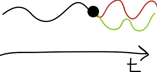
It is very difficult to filter data in real time because Fourier decomposition requires information about the entire dataset to properly fit a wave. To better understand this, look at the picture below. There is a timeseries where “now” is the big black dot. The red and green lines are two different possibilities (there are an infinite number of possibilities) of what the future might look like. If you were to try to fit a sine wave to these data, you’d have a problem! How do you know how to fit the area after the dot? What happens after the dot will affect the shape of the wave that is fit in the days right before the dot. This is a problem.
My website gets around this problem by not filtering real time data at all. I use a variation of Paul Roundy’s real time projection algorithm. In an overly simplified sense, here's how it works. Imagine a Kelvin wave. This algorithm takes the current data and looks at how well it matches the structure of Kelvin waves in the past. The closer it matches, the higher the amplitude of the Kelvin wave shown in the plots.
Low Pass Mode
My hovmollers and horizontal maps have different modes that can be overlayed to help you diagnose where certain equatorial waves are at a given time. In addition to the MJO, Kelvin, and ER waves which have been mentioned here, I also have a low pass filter. This is low frequency (>100 day) filter that does a good job tracking convection associated with ENSO. Low frequency convection shifts east and west depending on the state of the ocean below it. To first order (and I stress, this really is only a first order approach), areas of active low frequency convection imply areas of anomalously positive SSTs, and vice-versa.
Shallow Water Theory
Imagine that the Earth is covered in only a layer of water with a homogeneous density under hydrostatic balance. Let’s assume that the Coriolis force varies linearly (still zero at the Equator) instead of sinusoidally. Let’s call the depth of the water the equivalent depth. When the momentum equations are simplified to fit this ideal scenario and solved, an important set of solutions comes out which we call equatorial waves.
Although the real world is very different from the ideal world of shallow water theory, it is a decent approximation in the tropics and we see examples of equatorial waves all around us. Keep in mind that although I will talk only about the atmosphere here, these same wave modes can exist in the ocean as well.
Note, also, that the shallow water equations are non-convective (“dry”). In the real world we tend to focus on convectively coupled equatorial waves which are nothing more than the shallow water waves coupled to atmospheric convection. Convectively coupled waves move more slowly than dry waves.
Convectively coupled equatorial waves can be thought of as large scale areas that are especially conducive for convection. The presence of a CCEW does not necessarily imply convection and convection does not necessarily imply the presence of a CCEW.
The Kelvin Wave
The Kelvin wave is the simplest solution to the shallow water equations because it does not have a meridional wind component.
Special Properties: no meridional wind, must be trapped by something. In the real world Kelvin waves can be trapped by coastlines, mountains, or the equator.
Propagation Characteristics: Equatorially trapped convectively coupled Kelvin waves (the kind that we usually talk about) travel eastward at phase speeds of 15-20 m/s over the West Pacific and 12-15 m/s over the Indian Ocean because they tend to be more strongly coupled to convection. They are non-dispersive, so their group speed is equal to their phase speed.
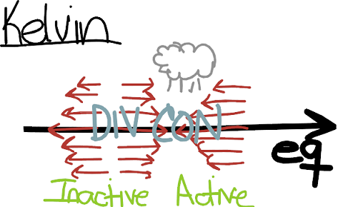
Horizontal Structure (see figure): Kelvin waves have their strongest zonal wind parallel to the equator which tapers off following a Gaussian function off the equator. They have a classic “in, up and out” structure with easterlies in front and westerlies in back. The area of zonal convergence in between is where the convection tends to occur. The area of convergence (associated with convection) is the “active” phase and the area of divergence (associated with suppressed vertical movement) is called the “inactive” phase.
Important Effects:
- Outflow from their convection can cause Rossby wave trains to develop. These aren’t as strong as the wave trains created by the MJO (read further) because Kelvin waves move so much faster.
- The westerly wind phase (back) of the of the Kelvin wave can be associated with westerly wind bursts (WWBs). These WWBs create stress on the ocean which can move warm water from the warm pool in the Pacific to the east, which is important for El Nino development.
- Kelvin waves travel through the MJO, and nearly every MJO event has a Kelvin wave at some point in its life. Most of the rainfall and PV generation within the MJO occurs within Kelvin waves that are moving through.
- Kelvin waves can provide favorable conditions for TCs to develop: convection, low-level vorticity, vertical shear and mid-level moisture.
The Equatorial Rossby Wave (ER)
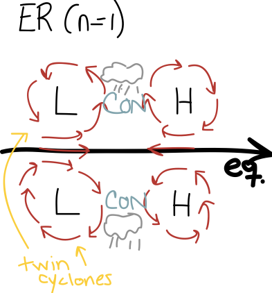
Special Properties: twin cyclones, equatorial symmetry, convection is displaced off the equator, can come in different “flavors”. Drawn below is an “n=1” ER wave, which is the most common. “n=2” ER waves can be spotted though. They are antisymmetric about the equator.
Propagation Characteristics: Travel westward at roughly 5 m/s.
Horizontal Structure: See below. The twin cyclones are one of the key aspects, as well as the location of the convection.
Important Effects:
- Outflow from their convection can cause Rossby wave trains to develop, similar to Kelvin Waves. ER waves are much more closely tied to midlatitude wave trains.
- The westerlies can be associated with westerly wind bursts, just like in the Kelvin wave.
- ER waves travel through the MJO, just like Kelvin waves do, and some might argue that they are a trigger for MJO intiation.
- Twin cyclones can spin off and become tropical depressions. The vorticity associated with the convection can lead to TC genesis.
The Madden Julian Oscillation (MJO)
The MJO is an envelope of convection that travels eastward around the Equator in about 30-60 days. It is often considered to “begin” in the Indian ocean.
Special Properties: larger scale than either Kelvin or ER waves, large area of active convection and broad wind fields can have significant impacts on the atmosphere and ocean, no theroetical basis. We don’t know what it is or why it exists.
Propagation Characteristics: “Starts” in the Indian Ocean and travels east at roughly 5 m/s. The convective signal tends to disappear over the Eastern Pacific, but the wind signals usually stick around and speed up as it decouples from convection.
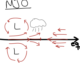
Horizontal Structure: See below. Looks a little like a hybrid of Kelvin and ER waves. This has not gone unnoticed in the literature. This is a difficult structure to draw because it varies so much as it goes around the globe. The picture below is just a rough idea. Note that the convection (active phase) is in the westerlies. The structure of the MJO is very dependent on the season and the state of ENSO. The ER-type back half disappears as the MJO moves over the warm pool.
Important Effects:
- The MJO is associated with nearly every kind of weather phenomenon you can think of. Below is a *small* sampling.
- Associated WWBs can be crucial for ENSO development. Since the MJO moves more slowly than Kelvin waves, the WWBs last longer and more warm water can be moved eastward as an MJO moves through the Central Pacific.
- Convection associated with the MJO can generate midlaitude wave trains, just like Kelvin waves.
- Many of the attributes that make Kelvin waves a favorable environment for TC genesis are also present in the MJO. See above for more details.
What is an atmospheric wave?
Before we can understand equatorial waves, we need to understand what an atmospheric wave is in the first place. At its core, an atmospheric wave is an oscillation in some atmospheric field(s). Most meteorologists are used to seeing Rossby waves in the midlatitudes which show up really well on isobaric geopotential height maps. These Rossby waves are oscillating patterns in the pressure (and therefore geopotential height) fields which propagate around the globe.
Basic Wave Properties
Just like the sinusoidal waves taught in math and physics classes, atmopsheric waves have very important properties: amplitude, wavelength, wavenumber, frequency, period, phase velocity and group velocity.
Amplitude: the amplitude of a wave is the amount that a wave deviates from its base state.
Wavelength: the wavelength of a wave in the atmosphere is the horizontal or vertical extent of the wave, measured from ridge-to-ridge or trough-to-trough.
Wavenumber: wavenumber is simply the number of waves you could fit around the globe, almost always measured in a longitudinal sense. For example, you can fit one oscillation (one ridge and one trough) of a wavenumber 1 disturbance around the globe. You can fit 2 oscillations (two ridges and two troughs) of a wavenumber 2 disturbance around the globe, etc.
Frequency: the frequency of a wave is the number of times a wave oscillates in a given amount of time. Frequency and wavelength are inversely related (for a given phase speed) – longer wavelengths are associated with higher frequencies and vice-versa.
Period: The period of wave is the amount of time it takes to complete one cycle. It is the recipirocal of frequency, so low frequency waves have long periods and vice-versa.
Phase velocity: the phase velocity of a wave is the speed and direction at which the wave propagates. Positive phase velocities usually refer to eastward moving waves and negative phase velocities refer to westward moving waves. The phase speed is just the magnitude of the phase velocity.
Group velocity: the group velocity of a wave is the speed and direction at which the wave envelope propagates. When the group speed and the phase speed are equal, we say that the wave is non-dispersive. Also of note is that energy (information) about the wave packet moves at the group velocity, not the phase velocity.
Fourier Decomposition/Filtering
Fourier decomposition is one of the best techniques to separate wave types in the atmosphere. Every well-behaved (math term, we don’t need to worry about it so much) pattern can be separated entirely into a combination of sine/cosine waves with different properties. In meteorology we usually decompose atmospheric flows into waves that have separate wavenumbers and frequencies. This is called filtering. An important property of fourier decomposition is that when the sines and cosines are added back together, the original field is re-created, exactly as it was.
The take home point behind filtering is that it allows us to extract the parts of a field, such as OLR, that have the same wavenumber and frequency properties as a particular type of wave. This allows us to focus only on the relevant parts of the field.
Empirical Orthogonal Function (EOF) Analysis
EOF (a.k.a. Principal Component Analysis [PCA]) is a statistical technique for extracting the spatial structure which represents the most variance in a dataset. For example, the mode representing the most variance in a total-field (not anomaly) dataset is usually the seasonal cycle. EOF analysis is almost always performed on anomalies for just this reason. The mode representing the most variance of SSTs in the equatorial Pacific is ENSO.
The EOF is the spatial structure and the Principal Component (PC) is the timeseries that corresponds to the EOF. Imagine that we have the first EOF of SSTs. We can compare that spatial structure to the spatial structure that has occured every day for which we have recorded SST data. The more similar to the EOF that the actual data looks, the greater the amplitude of its PC will be. One could use the first EOF of SSTs as an ENSO timeseries.
EOF analysis is very complicated because it is full of caveats and subtleties which can make it difficult to interpret. Below is a list of some of them.
- EOFs are mathematical constructs. They are the eigenvectors of the covariance matrix of the dataset. They do not have to represent physical modes. All because an EOF looks physical does not mean that it is. Extreme caution needs to be used when relating EOFs to physical modes.
- EOFs are orthogonal (uncorrelated) with each other. This means that the first EOF represents the spatial pattern that explains the most variance, but the second EOF represents the spatial pattern that explains the second most varianceconstrained to being orthogonal to the first EOF. This is important because EOFs are forced to be independent of each other even though in the real world we know that physical modes are almost always correlated. If the first EOF changes, the subsequent EOFs change also. The principal components associated with each EOF are also completely uncorrelated.
- Because EOFs are orthogonal (90 degree phase shift) to each other, two EOFs can be used to describe propagating patterns. This is analogous to plotting a graph of sin(x) vs. cos(x), you end up with a circular pattern.
Realtime Multivariate MJO Index (RMM Index)
The RMM index was created by Matt Wheeler and Harry Hendon (Bureau of Meteorology, Australia) in a paper from 2004. They use EOF analysis to track the MJO on a simple circular diagram.
This is a popular method of tracking the MJO because it is easy to visualize and simple to make. However, since we do not know what the MJO actually is, we need to be careful to interpret the RMM index simply as a convenient method of tracking the MJO. It does not necessarily represent the true structure of the MJO, and often it is confused by other equatorial waves.
The RMM index is created like this:
- Start with OLR and zonal wind anomalies at 850 mb and 200 mb averaged over the Equator from 15S-15N.
- Subract the linear relationship that these fields have with ENSO.
- Perform an EOF analysis of all three fields, combined.
- The first and second EOFs are orthogonal to each other and show a propagating pattern, as described above.
- Plot the principal components (RMMs) associated with the first two EOFs on a polar coordinate plot.
- Arbitrarily split the circle into 8 phases. There is nothing magical about 8 phases. It could be as many, or as few, phases as you’d like.
- The amplitude of the MJO is shown by the distance of the plot from the center of the circle. This is equivalent to the modulus of the PCs [that is: amplitude = sqrt(PC1.^2+PC2.^2)].
- When the MJO amplitude is greater than 1 (outside the smaller circle), we consider the MJO to be active. When it is less than 1 we consider it to be inactive. Again, the number 1 is completely arbitrary.